How to excel at Excel
index match, index match match, sumif and sumifs
by: Michael Scalamogna- Enterprise Solutions Consultant with Opal Business Solutions
Have you ever had to manually flip between two Excel sheets to search for information? When attempting to reconcile something or build a report template, flipping between sheets can get tedious. Did you know Excel has some powerful functions that can help you find and summarize information in other cells, sheets and even workbooks?
The internet has lots of sites and blogs that you can use to learn how to use Excel more efficiently, but I’ve found that most of the content out there is either poorly written, on a website that is filled with cookies/advertisements or described using an example that’s not relevant to a finance professional. I hope this blog post is none of those.
If you already understand the below functions, you probably don’t need to read this post. Go find someone you work with and share your Excel knowledge instead!
- Index Match
- Index Match Match (my favorite)
- Sumif
- Sumifs
Index Match
Notice that the vlookup is not on this list. I’m skipping vlookups because The index match function does everything the vlookup does and more. When dealing with a lot of data, the index match function runs faster. You can also look up columns to the left. Most importantly, once you understand the syntax it’s quicker to write.
When building a report for clients using payables data from GP, always confirm that the payables checks are reconciled to their checkbook subledger. Confirm that the dollar amounts matched each sheet.
This morning I was building a report for a customer using payables data from GP. Since I was dealing with payables checks I wanted to make sure it reconciled to their checkbook subledger. I had two sheets, both with check numbers and dollar amounts on them. I needed to make sure the dollar amounts matched in each sheet.
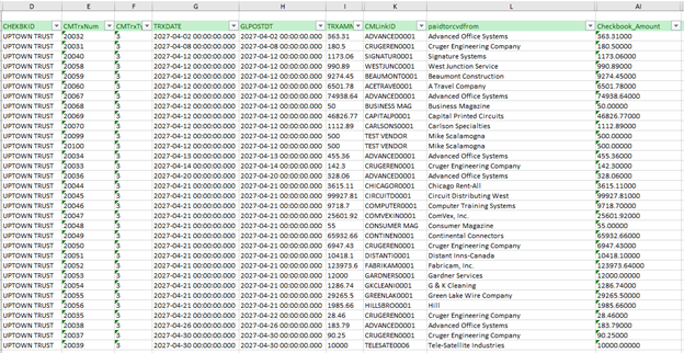
Figure 1: CMdata tab (Checkbook Data). The dollar amounts for comparison are in column AI and check numbers are in column E.
The sheet pictured above is from the checkbook in GP. I wanted to compare the dollar amounts in column AI to the corresponding dollar amounts from the accounts payable subledger.
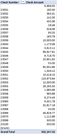
Figure 2: pmpivt sheet – AP Data summarized in a pivot table.
Figure 2 shoes AP data. I wanted to compare the “Check amount” column in Figure 2 to the “Checkbook_Amount” column in Figure 1.
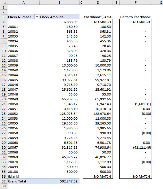
Figure 3: Reconciliation using INDEX MATCH formula
Columns D and F were added to the AP data added columns D and F to the AP data. The index match formula is in column D and shows the check $ amount from AP. Column F shows the difference between the check $ amount and the AP $ amount. Here is what my index match formula looked like:
=INDEX(cmdata!AI:AI,MATCH(pmpivt!A4,cmdata!E:E,0))
Or:
=index(CMdata column with check dollar amounts from figure 1 ,match( Payables check number from figure 3, CMdata column where the check numbers are from figure 1, I want the exact match))
In other words:
=index(values you want to find, match(cell on the current sheet that should have a match on the other sheet, column on the other sheet with a corresponding value, match type))
Index Match Match
This builds on the standard index match formula by adding another match function and enabling you to search for both a row AND a column. When I figured this out it took the top of my head off.
This is helpful when you have periodic financial data that you want to reference. I am going to use a simple example to explain. I have a monthly trial balance for last year on one tab. Rather than strain my eyes trying to find the net change for a specific account and time period, I can use the index match match function to do the work for me. You could expand on this idea and create a simple financial statement using a periodic trial balance.
Figure 4 is where I started.

Figure 4: A messy Excel sheet (“financial data” tab)
I want to have something like this:

Figure 5: Index match match making things easy for me (the “Switchboard”)
All I want to do is select the period ending date and the GL account number and see the period activity for that specific account.
Here is what the index match match formula looks like.
=INDEX(‘financial data’!C3:N9,MATCH(switchboard!E5,’financial data’!A3:A9,0),MATCH(switchboard!E3,’financial data’!C2:N2,0))
Or
=index( array on the financial data tab where the actual data lives excluding row titles and column headers from figure 4, match( GL account number on the switchboard from figure 5, column where GL account numbers are in the financial data tab from figure 4, I want an exact match), match( period end date on my switchboard from figure 5, array of possible period end dates from figure 4, I want an exact match))
In other words:
=index( array where actual data lives I want to return excluding row titles and column headers, match( row value I want to look up to find , vertical cell range where I want to search for the value, I want an exact match), match( value I want to look up to find the column, horizontal range where I want to find the value, I want an exact match))
This one also comes in handy when building a dashboard. You don’t want to see all the “raw data”, just the important pieces.
Sumif
Use sumif and sumifs to summarize numbers based on certain criteria. I recently helped one of our customers who had just acquired another company create prior year financials. The acquisition was official as of 1/1/2018. 2017 activity was not available in their instance of Dynamics GP so we created a consolidated 2017 monthly trial balance in Excel that we then linked to their Management Reporter reports.
I had the 2017 data all pulled together and available at the full account string level. I wanted to summarize the data to the natural account level and put it into a simple format that Management Reporter could read, so I used the sumif function to produce a consolidated trial balance. Here is a screenshot of what I started with:
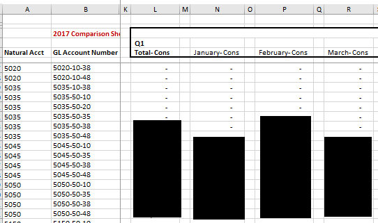
Figure 6: The starting point, “2017 Net Change Per Month” tab
Notice that I had a lot of accounts that would need combined if I wanted to see the data summarized at the natural account level. Below is a screenshot of the result:
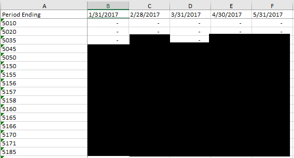
Figure 7: Sumif end result, “2017 Consolidated” tab
If you are reading this, you might wonder why I didn’t just use a pivot table to do this. I would have liked to use a pivot table, but the input data (figure 6) was not very pivot table friendly. I am sure I could have made it work with a pivot table, but I was just more comfortable using the sumif function.
Notice that in figure 6, account numbers 5035 and 5045 both needed to be summarized. Figure 7 shows the results of the sumif.
Here is what the sumif function looked like:
=sumif(‘2017 Net Change per Month’!A:A,’2017 Consolidated’!A145,’2017 Net Change per Month’!N:N)
Or:
=sumif(Column on net change tab with natural account numbers, cell in 2017 consolidated tab with natural account number to summarize, column in 2017 net change per month tab with dollar amounts to summarize)
Or:
=sumif( Grouping range , grouping criteria, the column with numbers that you want to summarize)
The sumifs function can be used if you have multiple criteria. It works largely the same, with one exception. The column that you want to summarize numbers by goes first, not last. The sumifs function would have looked like this:
=sumifs(‘2017 Net Change per Month’!N:N, ‘2017 Net Change per Month’!A:A,’2017 Consolidated’!A145)
Or:
=sumifs(column in figure 6 with dollar amounts to summarize, Column in figure 6 natural account numbers, cell in figure 7 with natural account number to summarize)
Or:
=sumifs(column with numbers you want to summarize, first grouping range, first grouping criteria, second grouping range, second grouping criteria)
These formulas have many different applications and can save you a lot of time. If you’re an Opal customer and have more questions about how these functions work, need help making sense of your data, or just have general Excel questions drop me a line at mscalamogna@opalbiz.com. I’m happy to help!
Questions?


